Measure Time of Flight to the Centimeter With PolarFire® Devices

How to Accomplish Time-Of-Flight Measurement in Our PolarFire^® FPGA

Modern autonomous robots, drones and vehicles need a precise view of their surroundings to safely navigate and move.

Light Detection and Ranging (LiDAR) sensors—where a laser scans the surroundings and measures the travel-time of a light pulse until a reflection returns for every measurement point—are commonly used for this purpose. Time-of-flight sensors are also readily available; however, increasing demand for fewer components within systems conflicts with the additional space and effort these devices require on a board.

Field Programmable Gate Arrays (FPGAs) are an ideal candidate for incorporating multiple functions into one device, especially given the calculations required for creating a point cloud out of individual measurement-results.

This blog post shows how a time-of-flight measurement can be accomplished in a Microchip PolarFire FPGA with a temporal resolution of 100 ps or less, equaling a distance-resolution of ~3 cm or less. This is achieved by using individual elements of carry chains which are abundantly present in FPGAs and comparing them against a known time-base of an internal free-running clock-signal.

The Basic Principle of Time-of-Flight Measurement

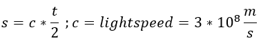
For time-of-flight measurements, laser pulses are emitted and directed by means of rotating mirrors or micro-electrical mechanical systems (MEMS) into a certain direction. By measuring the time until a reflection returns, one can calculate the distance to the reflecting object. As the measurement is the travel-time from the laser to the object and back, to calculate the distance calculation the measured time is halved.

Depending on the requirement of the system, distances of several meters up to several hundred meters need to be measured with distance accuracies of several centimeters. This results in measurement times down to the microsecond, with an accuracy in the 100-picosecond range. For example:

Minimum measurement range: 0.2 m
Maximum measurement range: 300 m
Distance resolution: 3 cm

Resulting timings:
Minimum measurement time:

Maximum measurement time:

Resolution:

An instant accuracy of 100 ps in an FPGA is typically achieved using multi-gigabit transceivers—in this example, running at 10 Gbps. However, these transceivers are a high-value component in an FPGA design and other means of measurement are preferred.

Measurement Using a Carry Chain

Very fast carry chains are present in Microchip FPGA architectures. The individual elements can be configured in multiple ways, one of them being a direct forwarding of an incoming signal FCI to FCO. The propagation delay is in the range of 10–30 ps and is not calibrated.

As the carry elements are very regular and are built for cascading, long chains of regular and small delays are possible. A thermometer approach of such a cascaded carry chain allows a fine-grained resolution of an incoming signal:

The returning photons of the reflected pulse are amplified outside the FPGA into a digital signal, which can be processed by the FPGA. The digital pulse is travelling through the uniform carry chain. On the rising edge of the sampling clock, the associated flip-flops will register the values of the individual taps of the delay chain, forming some temperature measurement pattern: the longer the duration, the further into the delay chain the 1 value has propagated. The sampling is an asynchronous crossing, hence at some flip-flops a setup-time violation will occur. On the following rising edge of the sample clock, the values from the first flip-flop stage are read into the second flip-flop stage to clean the asynchronous data crossing. The second set of flip-flops must be located physically as close as possible to their driving source. To guarantee this, physical location constraints are required, which are hard-placing these flip-flop pairs.

The initial reading of the thermometer measurement will look as follows:

Early pulse: 11111...111110000

Late pulse:  11100...000000000

Calibration and Accuracy

The carry elements are not calibrated, as they are built for short propagation delay. As the delay of the carry elements is short, many individual elements will be required for measuring delays in the nano-second range. Hence the data-sheet specification of 10–30 ps range/element needs to be more accurately known for measurement-purposes.

In semiconductor devices, specifications can vary widely over the production range. However, when using one single component, the variations are typically significantly smaller. This behavior is also used for narrowing down on the delay of the individual carry chain elements.

A clock signal of known frequency is sent into a delay-chain and the number of delay taps recorded, which are set. With the number of taps and the known duration of the clock, one can calculate the average delay of one single tap.

Example:

• Test-Clock: 350 MHz, i.e., period = ~2.86 ns, half-period = ~ 1.43 ns
• Tap delay:
• Min: 10 ps / delay-tap => 1.43 ns / 10 ps/tap => 143 taps
• Max: 30 ps / delay-tap => 1.43 ns / 30 ps/tap => 48 taps

Based on the number of “1” values in the delay chain, the average delay of one single delay can be calculated. Measurements at room temperature have shown delays around 18 ps/tap.

Very high accuracy requires a high number of individual taps, which often is not required, and a lower resolution is sufficient. To accommodate this, the delay chain for both calibration and measurement of the incoming signal is set up to tap off into flip-flops after a set number taps without a tap.

With six taps before a flip-flop, the 143 taps for the measurement of the half-period of the calibration clock is reduced to 24 visible bits, easing the handling and the measurement.

Time-of-Flight Measurement

In the initial paragraph about the working principle of time-of-flight measurements, the minimum and maximum timing for a given measurement range was calculated with the required precision.

To achieve those goals the measurement is split up in two parts:

• Coarse measurement for the measurement range
• Fine measurement, accurately aligned with the coarse measurement for the final resolution.

The coarse measurement is essentially done with a counter of the required size. This counter is started when a pulse is emitted and stopped by the incoming reflection.

Due to the flexibility of the FPGA, the counter can be easily built in the required resolution.

For our given example of 2000 ns maximum measurement time with a clock-period of 2.86 ns from the 350 MHz clock, the counter-size is:

2000 ns/ 2.86 ns/count = 700 count

Reaching a counter-value of 700 requires a 10-bit counter, which can reach a maximum value of 1023.

The fine measurement is performed using a second instance of the carry chain into which the reflected pulse travels. The number of carry elements that show a “1” signal is equivalent to the arrival time of the reflected pulse in comparison to the clock of the coarse measurement.

As the average tap delay of the carry element is known through the on-chip calibration, one can calculate the fine-grained measurement as:

Fine delay = (total number of visible taps) * delay/tap

The result of the fine measurement is added to the number of clock cycles of the coarse counter. For example:

• Coarse result: final counter value = 119
• Fine result: 24 visible taps
• 4 carry chain elements / capture flipflop
• Calibration result: 20 ps/tap

→ The measured example distance is between 102.666 cm and 102.690m

As components outside of the digital realm of the FPGA also add physical delay to the measurement, it is often advisable to perform measurements that cancel out these additional delays. This can be achieved by performing two measurements at the same time—one stopped when the light pulse leaves the system and one stopped by the returning pulse.

Detection of Multiple Echoes

An emitted laser pulse has a certain physical diameter and the reflections it causes may not be 100% uniform—that is, multiple echoes could return for a single transmitted pulse. These echoes can be relatively close together, and a very fast reactivation of the fine-grained measurement structure is required.

This is accomplished by transferring the detected values into independent FPGA registers for further processing. With this approach, the delay line can receive the next echo on the next clock cycle again.

Further Processing

LiDAR applications require the generation of a so-called point cloud, which contains information about the elevation, horizontal angle and distance of a measurement-point from the laser-scanner. Based on this, every measurement point is calculated into a 3D point, with X, Y and Z-coordinates.

The mathematics involved in these calculations are not part of this post; however, these are very suitable to be implemented in parallel on an FPGA fabric. This results in a relatively short latency for the creation of the 3D model.

In some applications adding embedded processing to the measurement device is beneficial from a performance-, cost- and size-perspective. The PolarFire System-on-Chip (SoC) FPGA, with its hardened RISC-V processing system, naturally lends itself to this task.

Conclusion

This post showed how Microchip FPGAs can be used to create a time-of-flight measurement with distance resolutions down to the centimeter range. This capability, combined with the high reliability, best-in-class performance/Watt and security up to military level, make them an excellent platform for reliable measurements. These devices address the “Big Three” usually required in every project:

1. Reduce Risk

With the flexible and highly power-efficient architecture of the PolarFire FPGA and SoCs fabric, future proof designs can be created that extend today’s architectures towards tomorrow’s requirements. Even though not explicitly described in this post, the high reliability and immunity to single event upsets make these devices an ideal candidate for demanding applications.

2. Save Money

Integration of functions into fewer devices allows to reduce the number of components on a board, allowing to create a physically smaller system.

3. Make Money

The flexibility of the FPGA allows a platform approach with a defined functionality that can be easily adopted to varying application requirements or end customers. With that, more markets are addressable with little development investment.

All in all, Microchip PolarFire SoC and FPGA are ideal candidates for use in automotive and industrial applications and meet the “Big Three” of your applications.